Load GW Data
Load-data.Rmd
library(beacon)
#>
#> Attaching package: 'beacon'
#> The following object is masked from 'package:utils':
#>
#>     vi
#> The following objects are masked from 'package:base':
#>
#>     mode, pipe
1. Download GW data from GWOSC
beacon employs GWOSC API (v2) to download the public GW
data. Therefore, you need the network connection.
There are helper functions, such as,
list_gwosc_event([##(1) Check available GW events])list_gwosc_param([##(3) Check parameters])
to check the right input for
download_*/get_* functions:
download_event([##(2) Download event data])get_gwosc_param([##(3) Check parameters])
(1) Check available GW events
GW_event_list <- list_gwosc_event()

cat("First 6 events:\n")
#> First 6 events:
print(head(GW_event_list))
#> [1] "GW240109_050431" "GW240107_013215" "GW240105_151143" "GW240104_164932"
#> [5] "GW231231_154016" "GW231231_120147"
(2) Download event data
Here we test with GW150914. Download event data using
download_event().
download_event(event_name = "GW150914", # event name
               det = "H1",              # Detector name
               path = "test_data/",     # download path
               file.format = 'hdf5',    # default
               sampling.freq = 4096     # default
               )

# YOU'LL SEE:
#
# > Trying event-level strain-files: https://gwosc.org/api/v2 /events/GW150914/strain-files
#   -> GET https://gwosc.org/api/v2/events/GW150914/strain-files
# > Downloading: https://gwosc.org/archive/data/O1/1126170624/H -H1_LOSC_4_V1-1126256640-4096.hdf5
#   -> to: test_data//H-H1_LOSC_4_V1-1126256640-4096.hdf5
# trying URL 'https://gwosc.org/archive/data/O1/1126170624/H -H1_LOSC_4_V1-1126256640-4096.hdf5'
# Content type 'application/octet-stream' length 130159479 bytes (124.1 MB)
# ==================================================
# downloaded 124.1 MB
If you want to:
- analyze data directly, and
- save your storage.
Set load=TRUE, and remove=TRUE . In this
case you don’t need to specify path (default path is
“./”).
(3) Check parameters
For available parameters, you can check by
param_names <- list_gwosc_param()

cat("First 6 parameters:\n")
#> First 6 parameters:
print(head(param_names))
#> [1] "GPS"                 "mass_1_source"       "mass_1_source_lower"
#> [4] "mass_1_source_upper" "mass_1_source_unit"  "mass_2_source"
Then collect parameter value(s) of specific event(s) as follows.
One parameter for an event:
params <- get_gwosc_param(
    name = 'GW150914',
    param = 'GPS'
)

cat("GPS time of GW150914:\n")
print(params) # returns 1x1 data.frame

# GPS time of GW150914:
#                 GPS
# GW150914 1126259462
Multiple parameters for an event:
params <- get_gwosc_param(
    name = 'GW150914',
    param = c('mass_1_source',
              'mass_2_source',
              'luminosity_distance',
              'GPS')
)

cat("Some parameters of GW150914:\n")
print(params) # returns 1x4 data.frame

# Some parameters of GW150914:
#          mass_1_source mass_2_source luminosity_distance        GPS
# GW150914          35.6          30.6                 440 1126259462
Or just all the available parameters for an event:
params <- get_gwosc_param(
    name = 'GW150914',
    param = 'all'
)

print(params) # returns 1x45 data.frame
#
#                 GPS mass_1_source mass_1_source_lower mass_1_source_upper mass_1_source_unit ...
# GW150914 1126259462          35.6                 3.1                 4.7              M_sun ...
#
2. Load HDF5 Data
Since R doesn’t have any package for reading gwf files
for the moment, we mainly treat hdf5 (or h5)
file format.
Using following functions, one can read and write hdf5
files:
read_H5write_H5
Basically those functions refer to the structure of hdf5
as follows.
meta/GPSstart: Starting GPS time of strain data is stored.strain/Strain: Strain data is stored.
Additionally, if GW data has a Data Quality (DQ), it will refer to:
-
quality/simple/DQmask: DQ mask of bits is stored in decimal unit.
(1) Read hdf5 file
For using simluated demo data for the illustration, it can be found in following directory:
demo.file <- system.file("extdata", "demo_4kHz.h5", package = "beacon")

cat('Demo hdf5 data file directory:\n')
#> Demo hdf5 data file directory:
print(demo.file)
#> [1] "/home/runner/work/_temp/Library/beacon/extdata/demo_4kHz.h5"
(The demo data was created by using Python’s pycbc
package)
read_H5 will load strain data and GPS start time to
construct ts object (here, you need to know the sampling
frequency, e.g. 4096 Hz).
demo <- read_H5(
    file = demo.file,
    sampling.freq = 4096,
    dq.level = 'all' # defulat: "BURST_CAT2"
)
cat(
    "Demo Data Summary:\n",
    "- Starting time:", ti(demo), "s\n",
    "- End time:", tf(demo), "s\n",
    "- Duration:", tl(demo), "s\n",
    "- Time range:", paste(tr(demo), collapse=' - '), "s\n",
    "- Sampling frequency:", frequency(demo), "Hz\n"
)
#> Demo Data Summary:
#>  - Starting time: 0 s
#>  - End time: 31.99976 s
#>  - Duration: 32 s
#>  - Time range: 0 - 31.999755859375 s
#>  - Sampling frequency: 4096 Hz
print(demo)
#> Time Series:
#> Start = c(0, 1)
#> End = c(31, 4096)
#> Frequency = 4096
#>  [1] -1.402802e-20 -1.451734e-20 -1.529089e-20 -1.461478e-20 -1.516181e-20
#>  [6] -1.447528e-20 -1.515767e-20 -1.474572e-20 -1.496885e-20 -1.535953e-20
#> [11] -1.498296e-20 -1.472902e-20 -1.564059e-20 -1.546743e-20 -1.471808e-20
#> [16] -1.587687e-20 -1.512821e-20 -1.579603e-20 -1.493327e-20 -1.541508e-20
#>  [ reached 'max' / getOption("max.print") -- omitted 131052 entries ]
#> attr(,"dqmask")
#>       DATA CBC_CAT1 CBC_CAT2 CBC_CAT3 BURST_CAT1 BURST_CAT2 BURST_CAT3
#>  [1,]    1        1        1        1          1          1          1
#>  [2,]    1        1        1        1          1          1          1
#>  [ reached 'max' / getOption("max.print") -- omitted 30 rows ]
#> attr(,"dqmask")attr(,"tsp")
#> [1]  0 31  1
#> attr(,"dqmask")attr(,"level")
#> [1] all
Plot oscillogram:
plot_oscillo(demo)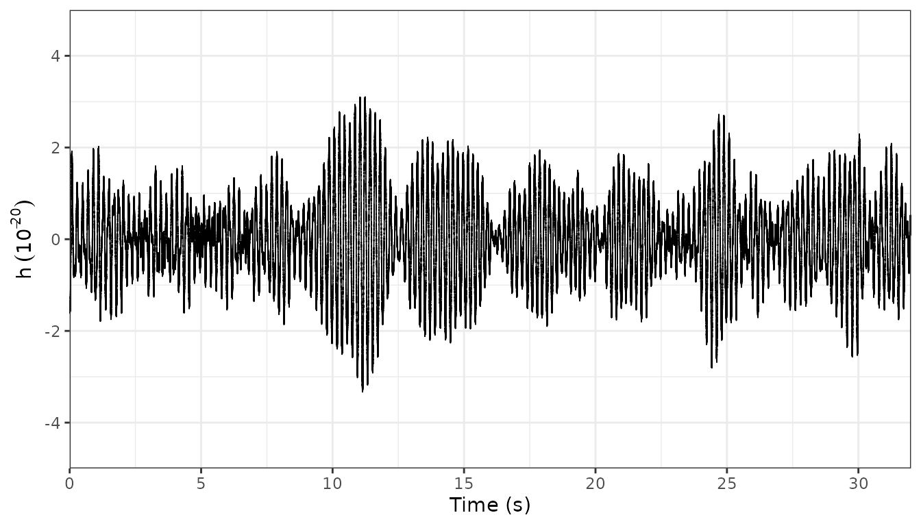
Using get_dqmask, you can extract the (multivariate)
time series of DQ bits with the sampling frequency of 1 Hz.
print(get_dqmask(demo))
#> Time Series:
#> Start = 0
#> End = 31
#> Frequency = 1
#>    DATA CBC_CAT1 CBC_CAT2 CBC_CAT3 BURST_CAT1 BURST_CAT2 BURST_CAT3
#>  0    1        1        1        1          1          1          1
#>  1    1        1        1        1          1          1          1
#>  [ reached 'max' / getOption("max.print") -- omitted 30 rows ]
#> attr(,"level")
#> [1] all
This will be used in DQ veto of BEACON pipeline.
(2) Write hdf5 file
Similarly to read_H5, write_H5 also refers
to basic directories of: meta/GPSstart, and
strain/Strain.
If you put more meta info, you can follow the code below:
write_H5(
    file = 'path/to/your/hdf5/file.h5',
    demo,
    meta.list =
        list(
            'meta/sample_freq' = frequency(demo),
            'quality/simple/DQmask' = rep(127, # All 1 of bit
                                          32)  # 32 s data case
        )
)
⚠️ Note: In current version,
read_H5does not read all the meta information in hdf5 file’s directory.